Chemical Reactor

We consider a single first-order, irreversible chemical reaction in an isothermal CSTR

\[A \to B.\]

The material balances and the system data are provided in [DAR11] and is given by the discrete time nonlinear model

\begin{equation*} \begin{split} c_{A}(k+1)&=c_{A}(k)+h\left(\frac{Q(k)}{V}(c_f^{A}-c_{A}(k))-k_r{c_{A}(k)}\right)\\ c_{B}(k+1)&=c_{B}(k)+h\left(\frac{Q(k)}{V}(c_f^{B}-c_{B}(k))+k_r{c_{B}(k)}\right), \end{split} \end{equation*}

in which \(c_A\geq 0\) and \(c_B\geq 0\) are the molar concentrations of \(A\) and \(B\) respectively, \(Q\leq 20\) (L/min) is the flow through the reactor and \(h\) is the sampling rate in minutes. The constants and their meanings are given in table below.

Reactor constants
		value	unit
feed concentration of \(A\)	\(c_f^{A}\)	1	mol/L
feed concentration of \(B\)	\(c_f^{B}\)	0	mol/L
volume of the reactor	\(V_R\)	10	L
rate constant	\(k_r\)	1.2	L/(mol min)
sampling rate	\(h\)	0.5	min
initial value	\((c_0^{A},c_0^B)\)	\((0.4, 0.2)\)

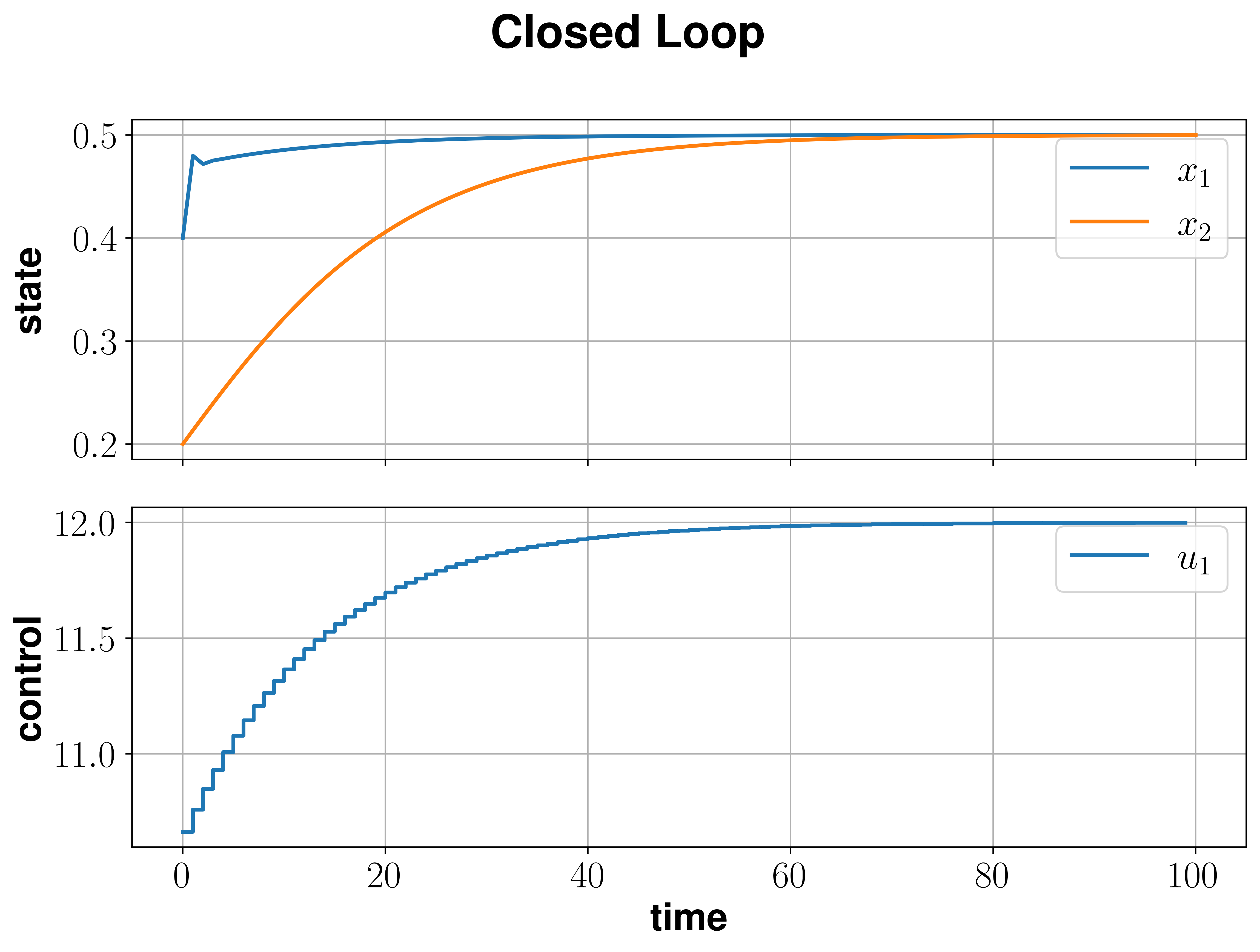
From this set of parameters we can compute the equilibrium \((c_e^{A},c_e^B,Q_e) = (\frac 1 2, \frac 1 2, 12)\) of the system.

To initialize the system dynamics a function that implements \(f(x,u)\), where \(x = (c_{A},c_{B})^T\) and \(u=Q\) has to be defined.

V = 10.
cf_A = 1.
cf_B = 0.
k_r = 1.2
h = 0.5

def f(x,u):
    y = nmpyc.array(2)
    y[0] = x[0] + h*((u[0]/V) *(cf_A - x[0]) - k_r*x[0])
    y[1] = x[1] + h*((u[0]/V) *(cf_B - x[1]) + k_r*x[1])
    return y

After that, the nMPyC system object can be set by calling

system = nmpyc.system(f, 2, 1, system_type='discrete')

In the next step, the objective is defined by using the stage cost given by

\begin{align*} \ell (c_{A}(k),c_{B}(k),Q(k))&=\frac 1 2\vert c_A(k)-\frac 1 2\vert^2+\frac 1 2 \vert c_B(k)-\frac 1 2\vert^2+\frac 1 2 \vert Q(k) -12 \vert^2\\ \end{align*}

Since we do not need terminal cost, we can initialize the objective directly using the following implementation.

def l(x,u):
    return 0.5 * (x[0]-0.5)**2 + 0.5 * (x[1]-0.5)**2 + 0.5 * (u[0]-12)**2

objective = nmpyc.objective(l)

In terms of the constraints we assume that

\[\begin{split}0 &\leq x_1(k) & < \infty & \quad & \text{for } k=0,\ldots,N \\ 0 &\leq x_2(k) & < \infty & \quad & \text{for } k=0,\ldots,N \\ 0 &\leq u(k) & \leq 20 & \quad & \text{for } k=0,\ldots,N-1.\end{split}\]

This can be realized in the code as follows:

constraints = nmpyc.constraints()
lbx = nmpyc.zeros(2)
ubu = nmpyc.ones(1)*20
lbu = nmpyc.zeros(1)
constraints.add_bound('lower','state', lbx)
constraints.add_bound('lower','control', lbu)
constraints.add_bound('upper','control', ubu)

Moreover, we consider the equilibrium \((c_e^{A},c_e^B,Q_e)\) as th terminal condition for our optimal control problem, which is implemented as

xeq = nmpyc.array([0.5,0.5])
def he(x):
    return x - xeq
constraints.add_constr('terminal_eq', he)

After all components of the optimal control problem have been implemented, we can now combine them into a model and start the MPC loop. For this Purpose, we define

\[x(0) = (0.4,0.2)^T\]

and set \(N=15\), \(K=100\).

model = nmpyc.model(objective,system,constraints)
x0 = nmpyc.array([0.4,0.2])
res = model.mpc(x0,15,100)

Following the simulation we can visualize the results by calling

res.plot()

which generates the plot bellow.