Heat Pump
This example describes a home heating system that involves the optimal control of a small heat pump coupled to a floor heating system. The corresponding dynamic model is introduced in [LHDI10] and is given by
where \(x_1\) denotes the temperature of the water returning from the heating, \(x_2\) denotes the room temperature and \(u\) is the heat supplied from the heat pump to the floor. Further, the ambient temperature
describes a sinusoidal disturbance from the outside temperature where \(t_f = 24\). The remaining constants are summarized in the table below.
Reactor constants |
|||
|---|---|---|---|
|
value |
unit |
|
density of the water |
\(\rho_W\) |
997 |
\(kg/m^3\) |
specific heat capacity of water |
\(c_W\) |
4.1851 |
\(J/kgK\) |
volume of the water |
\(V_H\) |
7.4 |
\(m^3\) |
thermal conductivity between water and the room |
\(k_{WR}\) |
510 |
\(W/K\) |
thermal conductivity between the room and the environment |
\(k_G\) |
125 |
\(W/K\) |
thermal time constant of the room |
\(\tau_G\) |
260 |
\(s\) |
First, we have to implement the outside temperature in the code to define our system dynamics.
t_f = 24
def T_amb(t):
 return 2.5 + 7.5*nmpyc.sin((2*nmpyc.pi*t)/t_f - (nmpyc.pi/2))
After that, we can define the right hand side of the system by
rho_W = 997
c_W = 4.1851
V_H = 7.4
k_WR = 510
k_G = 125
thau_G = 260
def f(t,x,u):
   y = nmpyc.array(2)
   y[0] = (-k_WR/(rho_W*c_W*V_H)*x[0]
            + k_WR/(rho_W*c_W*V_H)*x[1]
            + 1/(rho_W*c_W*V_H)*u[0])
   y[1] = (k_WR/(k_G*thau_G)*x[0]
            - (k_WR + k_G)/(k_G*thau_G)*x[1]
            + (1/thau_G)*T_amb(t))
   return y
And finally initialize the system by
system = nmpyc.system(f, 2, 1, 'continuous', sampling_rate=0.5, method='euler')
In the heating system the conflict between energy and thermal comfort arises. Thus, the stage cost reads
where \(P_{\max} = 15000 (W)\) is the maximal power of the heating pump and \(T_\text{ref} = 22^{\circ} C\) is the desired temperature of the room. The reference temperature \(T_\text{ref}\) can be selected differently – depending on the individual thermal comfort.
According to this we can initialize our objective by
P_max = 15000
T_ref = 22
def l(x,u):
   return (u[0]/P_max) + (x[1]-T_ref)**2
and implement the control constraint
as
constraints = nmpyc.constraints()
constraints.add_bound('lower', 'control', nmpyc.array([0]))
constraints.add_bound('upper', 'control', nmpyc.array([P_max]))
After all components of the optimal control problem have been implemented, we can now combine them into a model and start the MPC loop. For this purpose, we define
and set \(N=30\) and \(K=500\).
model = nmpyc.model(objective,system,constraints)
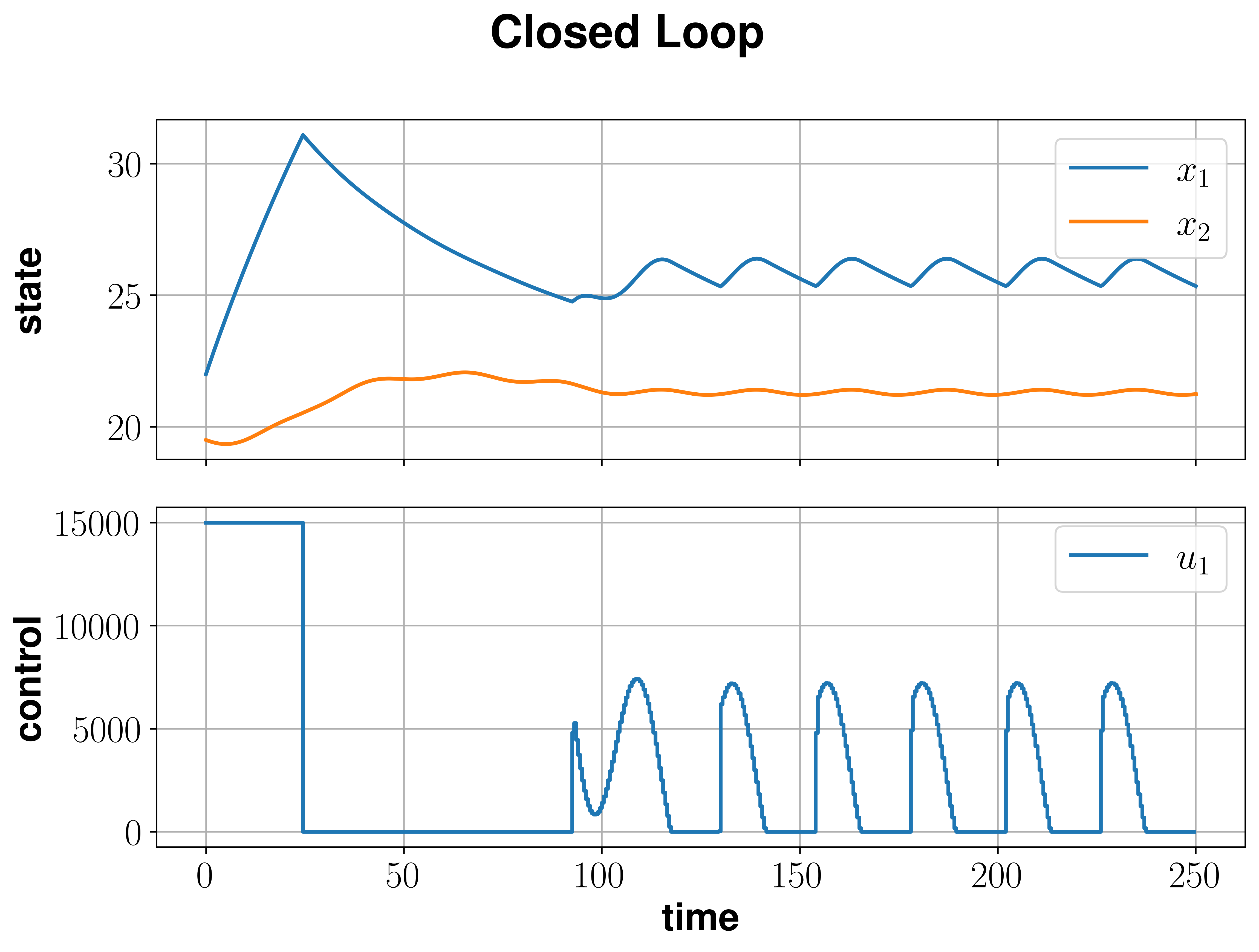
x0 = nmpyc.array([22., 19.5])
res = model.nmpyc(x0,N,K)
Following the simulation we can visualize the results by calling
res.plot()
which generates the plot bellow.